Introduction to Spatial data in R

R and RStudio

To avoid problems, please start by updating your installation of R to the latest version. Installers for R can be found here https://cloud.r-project.org/

Download the most recent version of RStudio at https://www.rstudio.com/products/rstudio/download/.

Library installation

In this tutorial, we will work with three libraries:

• sp: for working with vector data,
• rgdal: for importing and exporting vector data from other programs,
• raster: for working with raster data,
• tidyverse: for data wrangling (optional).

On Windows:

Just run: install.packages(c("sp", "raster", "rgdal"))

On Mac:

First download and install GDAL complete

If everything went well, the following three commands should run without problem!

    library(sp)
    library(rgdal)

## rgdal: version: 1.3-9, (SVN revision 794)
##  Geospatial Data Abstraction Library extensions to R successfully loaded
##  Loaded GDAL runtime: GDAL 2.3.2, released 2018/09/21
##  Path to GDAL shared files: /usr/share/gdal
##  GDAL binary built with GEOS: TRUE 
##  Loaded PROJ.4 runtime: Rel. 5.1.0, June 1st, 2018, [PJ_VERSION: 510]
##  Path to PROJ.4 shared files: (autodetected)
##  Linking to sp version: 1.3-1

    library(raster)

## 
## Attaching package: 'raster'

## The following object is masked from 'package:dplyr':
## 
##     select

## The following object is masked from 'package:tidyr':
## 
##     extract

Spatial Data in R

Almost all spatial structures in R are based on the sp package. There are three main types of spatial data we’ll work with: points, lines, and polygons.

There are three basic steps to creating spatial data by hand:

• Create geometric objects (points, lines, or polygons)
• Convert those geometric objects to Spatial* objects (* stands for Points, Lines, or Polygons)

To make them spatial objects, we also need to include information on how those x-y coordinates relate the places in the real world using a Coordinate Reference System (CRS).

First Spatial* Object: SpatialPoints

Points are the most basic geometric shape, so we begin by building a SpatialPoints object.

A points is defined by a pair of x-y coordiantes, so we can create a set of points by (a) creating matrix of x-y points, and (b) passing them to the SpatialPoints function to create our first SpatialPoints object.

coordinates <- rbind(c(1.5, 2.00),
                     c(2.5, 2.00), 
                     c(0.5, 0.50), 
                     c(1.0, 0.25), 
                     c(1.5, 0.00), 
                     c(2.0, 0.00), 
                     c(2.5, 0.00), 
                     c(3.0, 0.25), 
                     c(3.5, 0.50)) 

spatial.points <- SpatialPoints(coordinates) 
# ..converted into a spatial object
plot(spatial.points)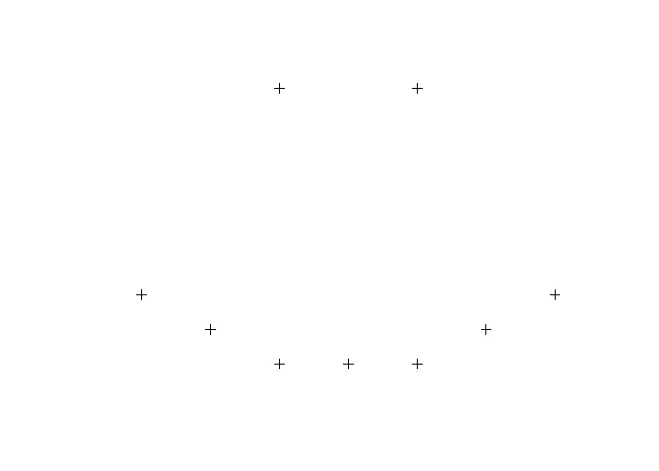

To get a summary of how R sees these points, we can ask it for summary information in a couple different ways. Here’s a summary of available commands:

summary(spatial.points)

## Object of class SpatialPoints
## Coordinates:
##           min max
## coords.x1 0.5 3.5
## coords.x2 0.0 2.0
## Is projected: NA 
## proj4string : [NA]
## Number of points: 9

coordinates(spatial.points)

##       coords.x1 coords.x2
##  [1,]       1.5      2.00
##  [2,]       2.5      2.00
##  [3,]       0.5      0.50
##  [4,]       1.0      0.25
##  [5,]       1.5      0.00
##  [6,]       2.0      0.00
##  [7,]       2.5      0.00
##  [8,]       3.0      0.25
##  [9,]       3.5      0.50

Terminology

1. Projection: Among cartographers, the term “projection” is synonymous with Flattening Function. All Flattening Functions are referred to as projections. However, in some programs (like ArcGIS), the term projection (or the term Projected Coordinate System) is used to refer to a bundle that includes both a Globe Model and a Flattening Model.
2. Coordinate Reference System (CRS): CRS is the term used by GIS packages in R to define both a Globe Model and a Flattening Model.
3. Projected Coordinate System: The ArcGIS term for a bundle of both a Globe Model and a Flattening Model
4. Geographic Coordinate System: The ArcGIS term for just a Globe Model. If you specify a Geographic Coordinate System but not a Projected Coordinate System, ArcGIS will often refuse to execute certain tools. However, it will still show you an image of your data, often by just using a Plate Carrée projection.

CRS objects can be created by passing the CRS() function the code associated with a known projection. You can find the codes for most commonly used projections from www.spatialreference.org or https://epsg.io/.

The most commonly used CRS is the WGS84 latitude-longitude projection. You can create a WGS84 lat-long projection object by either passing the reference code for the projection – CRS("+init=EPSG:4326") – or by directly calling all its relevant parameters – CRS("+proj=longlat +ellps=WGS84 +datum=WGS84 +no_defs").

is.projected(spatial.points) # see if a projection is defined. 

## [1] NA

crs.geo <- CRS("+init=epsg:32633")  # looks up UTM 33N
proj4string(spatial.points) <- crs.geo  # define projection system of our data
is.projected(spatial.points)

## [1] TRUE

summary(spatial.points)

## Object of class SpatialPoints
## Coordinates:
##           min max
## coords.x1 0.5 3.5
## coords.x2 0.0 2.0
## Is projected: TRUE 
## proj4string :
## [+init=epsg:32633 +proj=utm +zone=33 +datum=WGS84 +units=m +no_defs
## +ellps=WGS84 +towgs84=0,0,0]
## Number of points: 9

When CRS is called with only an EPSG code, R will try to complete the CRS with the parameters looked up in the EPSG table:

crs.geo <- CRS("+init=epsg:32633")  # looks up UTM 33N
crs.geo # prints all parameters

## CRS arguments:
##  +init=epsg:32633 +proj=utm +zone=33 +datum=WGS84 +units=m +no_defs
## +ellps=WGS84 +towgs84=0,0,0

Add Attributes

Moving from a SpatialPoints to a SpatialPointsDataFrame occurs when you add a data.frame of attributes to the points. Let’s just add an arbitrary table to the data – this will label each point with a letter and a number.

Note points will merge with the data.frame based on the order of observations.

df <- tibble(attr1 = letters[1:9],  # needs tidyverse library
                 attr2 = c(101:109))
glimpse(df)

## Observations: 9
## Variables: 2
## $ attr1 <chr> "a", "b", "c", "d", "e", "f", "g", "h", "i"
## $ attr2 <int> 101, 102, 103, 104, 105, 106, 107, 108, 109

first.spdf <- SpatialPointsDataFrame(spatial.points, df)
summary(first.spdf)

## Object of class SpatialPointsDataFrame
## Coordinates:
##           min max
## coords.x1 0.5 3.5
## coords.x2 0.0 2.0
## Is projected: TRUE 
## proj4string :
## [+init=epsg:32633 +proj=utm +zone=33 +datum=WGS84 +units=m +no_defs
## +ellps=WGS84 +towgs84=0,0,0]
## Number of points: 9
## Data attributes:
##     attr1               attr2    
##  Length:9           Min.   :101  
##  Class :character   1st Qu.:103  
##  Mode  :character   Median :105  
##                     Mean   :105  
##                     3rd Qu.:107  
##                     Max.   :109

Now that we have attributes, we can also subset our data the same way we would subset a data.frame. Some subsetting:

first.spdf[1:2, "attr1"] # row 1 and 2 only, attr1

## class       : SpatialPointsDataFrame 
## features    : 2 
## extent      : 1.5, 2.5, 2, 2  (xmin, xmax, ymin, ymax)
## coord. ref. : +init=epsg:32633 +proj=utm +zone=33 +datum=WGS84 +units=m +no_defs +ellps=WGS84 +towgs84=0,0,0 
## variables   : 1
## names       : attr1 
## min values  :     a 
## max values  :     b

SpatialPoint from a lon/lat table

A SpatialPointsDataFrame object can be created directly from a data.frame by specifying which columns contain the coordinates.

This is interesting, for example if you have a spreadsheet that contains latitude, longitude and some values. You can read this into a data frame with read.table, and then create the object from the data frame in one step by using the coordinates() command. That automatically turns the dataframe object into a SpatialPointsDataFrame.

Example

URL: http://ourairports.com/countries/EC/airports.hxl

airports <- read_csv("data/ec-airports.csv", comment = "##")

## Parsed with column specification:
## cols(
##   .default = col_character(),
##   id = col_double(),
##   latitude_deg = col_double(),
##   longitude_deg = col_double(),
##   elevation_ft = col_double(),
##   scheduled_service = col_double(),
##   score = col_double(),
##   last_updated = col_datetime(format = "")
## )

## See spec(...) for full column specifications.

coordinates(airports) <- c("longitude_deg", "latitude_deg")
plot(airports)

URL: http://ourairports.com/countries/EC/airports.hxl

airports <- read_csv("data/ec-airports.csv", comment = "##")

## Parsed with column specification:
## cols(
##   .default = col_character(),
##   id = col_double(),
##   latitude_deg = col_double(),
##   longitude_deg = col_double(),
##   elevation_ft = col_double(),
##   scheduled_service = col_double(),
##   score = col_double(),
##   last_updated = col_datetime(format = "")
## )

## See spec(...) for full column specifications.

coordinates(airports) <- c("longitude_deg", "latitude_deg")
plot(airports)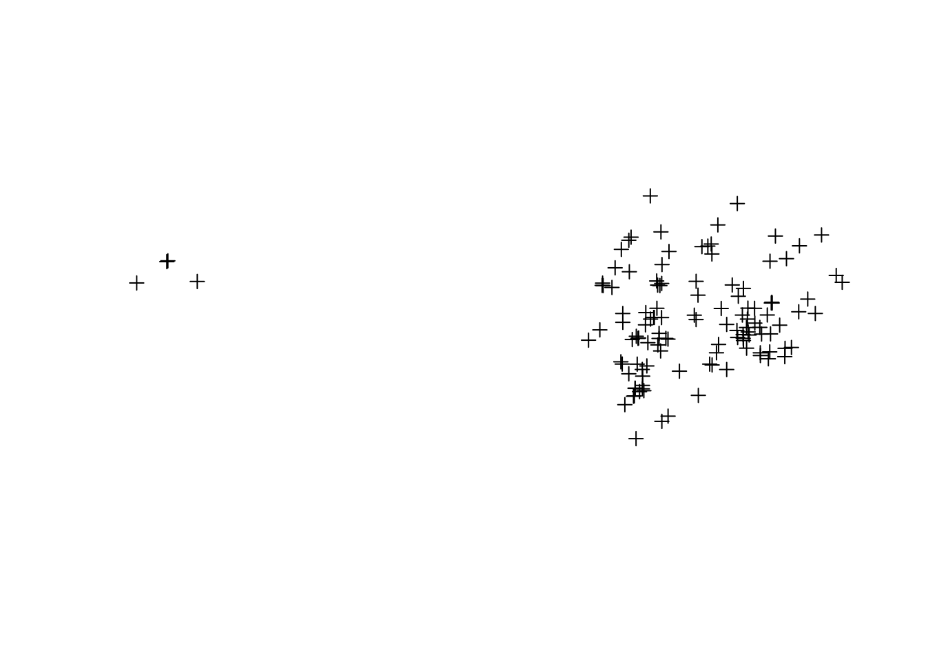

library(leaflet)
leaflet() %>% addTiles() %>% addMarkers(data = airports, 
                                        popup = ~municipality)

SpatialPolygons

To get a SpatialPolygons object, we have to build it up by:

1. creating Polygon objects,
2. combining those into Polygons objects, and finally
3. combining those to create SpatialPolygons.

• A Polygon object is a single geometric shape (e.g. a square, rectangle, etc.) defined by a single uninterrupted line around the exterior of the shape.
• A Polygons object consists of one or more simple geometric objects (Polygon objects) that combine to form what you think of as a single unit of analysis (an “observation”).
• A SpatialPolygons object is a collection of Polygons objects, where each Polygons object is an “observation”.

If you’re familiar with shapefiles, SpatialPolygons is basically the R analogue of a shapefile or layer.

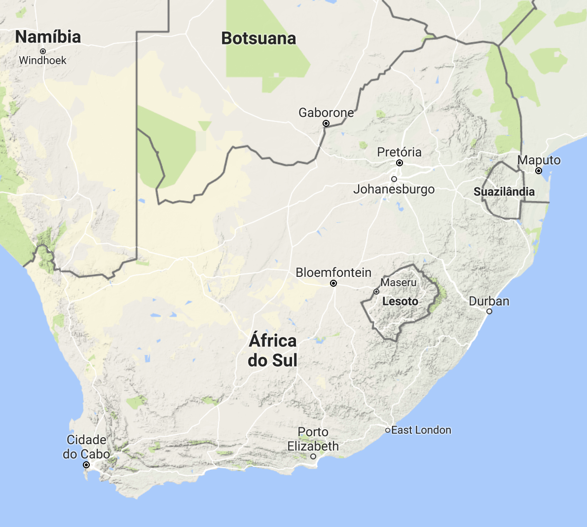
South Africa

SpatialPolygons object is a bit harder, but stil relatively straightforward with the spPolygons functions (from the raster package).

crdref <- CRS('+proj=longlat +datum=WGS84')
lon <- c(-116.8, -114.2, -112.9, -111.9, -114.2, -115.4, -117.7)
lat <- c(41.3, 42.9, 42.4, 39.8, 37.6, 38.3, 37.6)
lonlat <- cbind(lon, lat)
pols <- spPolygons(lonlat, crs=crdref)
pols

## class       : SpatialPolygons 
## features    : 1 
## extent      : -117.7, -111.9, 37.6, 42.9  (xmin, xmax, ymin, ymax)
## coord. ref. : +proj=longlat +datum=WGS84 +ellps=WGS84 +towgs84=0,0,0

We can make use generic R function plot to make a map.

pts <- SpatialPoints(lonlat)
plot(pols, axes=TRUE, las=1)
plot(pols, border='blue', 
     col='yellow', lwd=3, 
     add=TRUE)
points(pts, col='red', 
       pch=20, cex=3)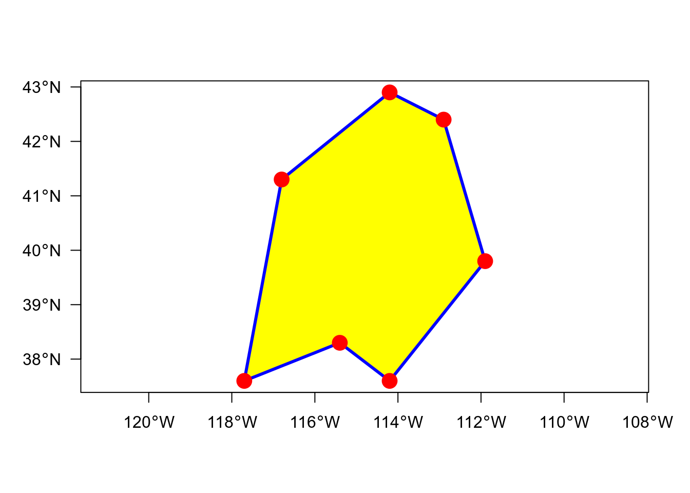

leaflet() %>% addTiles() %>% addCircleMarkers(data = pts, color = "red") %>% 
  addPolygons(data = pols, color = "blue", fillColor = "yellow")

# create polyon objects from coordinates
Sr1 <- Polygon(cbind(c(2, 4, 4, 1, 2), c(2, 3, 5, 4, 2)))
Sr2 <- Polygon(cbind(c(5, 4, 2, 5), c(2, 3, 2, 2)))
Sr3 <- Polygon(cbind(c(4, 4, 5, 10, 4), c(5, 3, 2, 5, 5)))
Sr4 <- Polygon(cbind(c(5, 6, 6, 5, 5), c(4, 4, 3, 3, 4)), hole = TRUE)

# create lists of polygon objects from polygon objects and unique ID
Srs1 <- Polygons(list(Sr1), "s1")
Srs2 <- Polygons(list(Sr2), "s2")
Srs3 <- Polygons(list(Sr3, Sr4), "s3/4")

# create spatial polygons object from lists
SpP <- SpatialPolygons(list(Srs1, Srs2, Srs3), 1:3)

plot(SpP)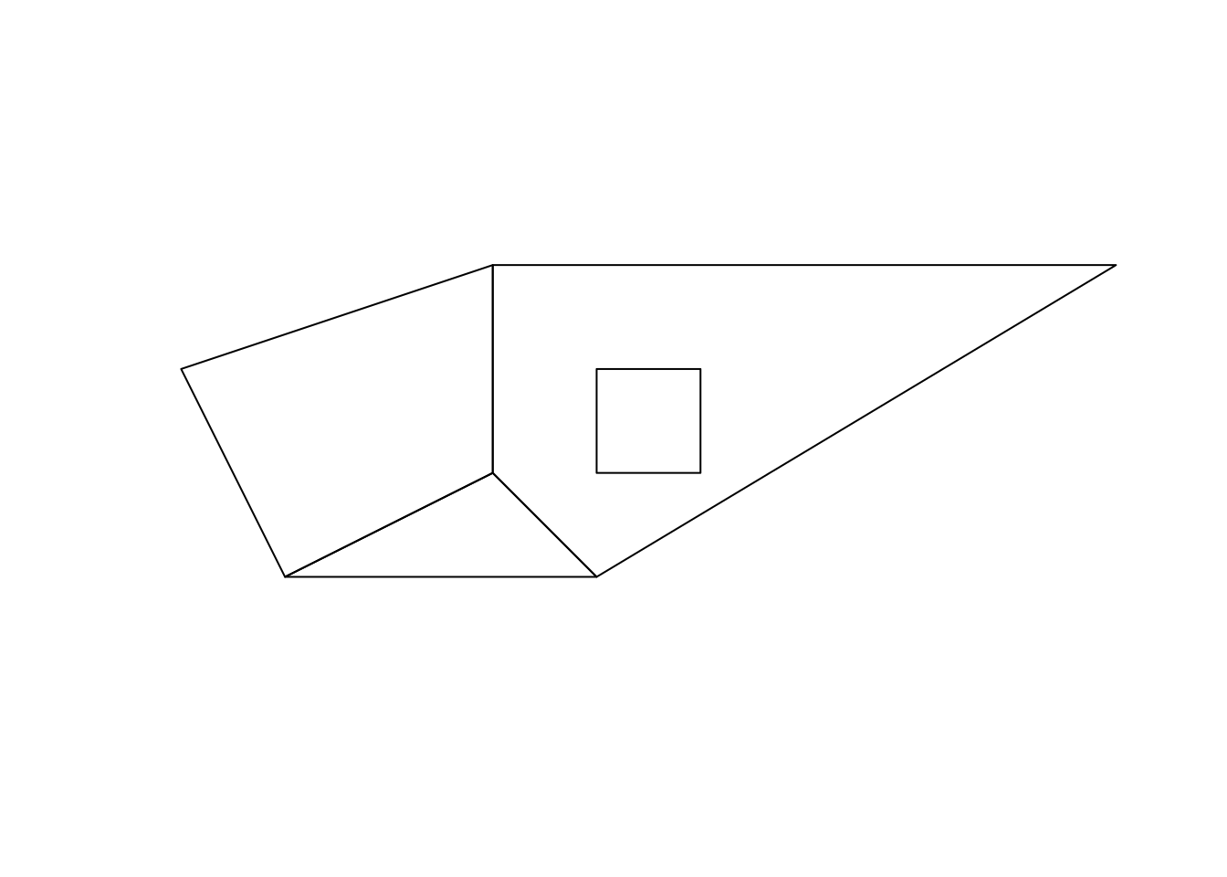

SpatialPolygonsDataFrame

attr <- data.frame(numbers = 1:3, 
                   characters = LETTERS[3:1], 
                   row.names = c("s3/4", "s1", "s2"))
SpDf <- SpatialPolygonsDataFrame(SpP, attr)

spplot(SpDf)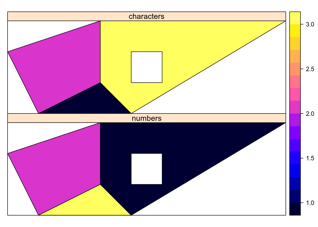

SpatialLines objects are basically like SpatialPolygons, except they’re built up using Line objects (each a single continuous line, like each branch of a river), Lines objects (collection of lines that form a single unit of analysis, like all the parts of a river), to SpatialLines (collection of “observations”, like rivers).

SRTM, Worldclim, Global adm. boundaries

The raster package is a great tool for raster processing and calculation but also very useful for data acquisition. With the function getData() you can download the following data directly into R:

• SRTM 90 — The Shuttle Radar Topography Mission (elevation data with 90m resolution between latitude -60 and 60).
• World Climate Data (Tmin, Tmax, Precip, BioClim)
• Global adm. boundaries (different levels)

Administrative boundaries

library(raster)
ecuador_level0 <- getData('GADM', country='ECU', level=0)
glimpse(ecuador_level0)

## Formal class 'SpatialPolygonsDataFrame' [package "sp"] with 5 slots
##   ..@ data       :'data.frame':  1 obs. of  2 variables:
##   .. ..$ GID_0 : chr "ECU"
##   .. ..$ NAME_0: chr "Ecuador"
##   ..@ polygons   :List of 1
##   .. ..$ :Formal class 'Polygons' [package "sp"] with 5 slots
##   ..@ plotOrder  : int 1
##   ..@ bbox       : num [1:2, 1:2] -92.01 -5.02 -75.19 1.68
##   .. ..- attr(*, "dimnames")=List of 2
##   ..@ proj4string:Formal class 'CRS' [package "sp"] with 1 slot

GADM: Ecuador Level 0

ecuador_level0 %>% leaflet() %>% addTiles() %>%  
  addPolygons(col = "blue", fillColor = "yellow", weight = 1.5)

library(raster)
paraguay_level1 <- getData('GADM', country='PRY', level=1)
paraguay_level2 <- getData('GADM', country='PRY', level=2)

paraguay_level1 %>% leaflet() %>% 
  addTiles() %>%  
  addPolygons(col = "blue", weight = 1,
              fillColor = "yellow")

paraguay_level2 %>% leaflet() %>% 
  addTiles() %>%
  addPolygons(col = "red", weight = 1,
              fillColor = "yellow")

Spatial* objects: @ vs $ access

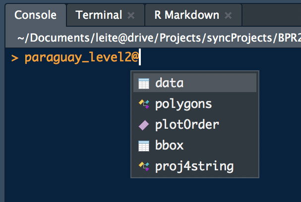
RStudio screenshot

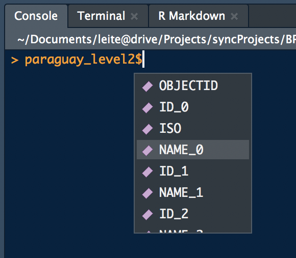
RStudio screenshot

Other I/O commands

# read/write shapefiles (and others)
#  - list formats
ogrDrivers()
dsn <- "path_to_shapefile"
ogrListLayers(dsn)
ogrInfo(dsn)
ogrInfo(dsn=dsn, layer="cities")
shapes = readOGR(".", "data")
writeOGR(obj = shapes, dsn = ".", 
         layer = "data", 
         driver =  "ESRI Shapefile")
writeOGR(obj = shapes, 
         dsn =  "towns.kml",
         layer =  "towns", 
         driver =  "KML")

# -- rasters
# creates SpatialGrid objects
r = readGDAL("data.tif")

# Rasters/Brick objects from files
r = raster("data.tif")
# - write Raster to GeoTIFF
writeRaster(r, "data2.tif", "GTiff")
# - supported formats
writeFormats()
# or for Google Earth
KML(r, "r.kmz")

Subsetting

cerrito <- subset(paraguay_level2, paraguay_level2$NAME_2 == "Cerrito") # or
cerrito <- paraguay_level2[paraguay_level2$NAME_2 == "Cerrito",]
cerrito %>% leaflet() %>% addPolygons() %>% addTiles() # Plot

Toy example

Calculate the proportion of forest in 10 random buffers across a landscape. Let’s first generate the landscape.

set.seed(123)
library(rgdal)
library(raster)
library(rgeos)

## rgeos version: 0.4-2, (SVN revision 581)
##  GEOS runtime version: 3.6.2-CAPI-1.10.2 
##  Linking to sp version: 1.3-1 
##  Polygon checking: TRUE

library(tidyverse)
uruguay <- getData('GADM', country='URY', level=0)
uruguay_projected <- spTransform(uruguay, CRS("+init=epsg:3857"))
forest_projected <- uruguay_projected %>% 
  spsample(200, type = "random") %>% 
  # build random poisson buffers around them
  gBuffer(width = 4000*rpois(length(.), 4), byid = TRUE) %>% 
  gEnvelope(byid = TRUE) %>% # take their envelope
  gUnaryUnion()

forest_projected <- gIntersection(uruguay_projected, forest_projected)
forest <- spTransform(forest_projected, CRSobj = crs(uruguay))

Toy example: Landscape

map<- leaflet() %>% addTiles() %>% 
  addPolygons(data = uruguay, weight = 1) %>% 
  addPolygons(data = forest, weight = 1, 
              fillColor = "green", 
              color = "darkgreen", popup = "Some beautiful shape")
map

Toy Example: Solution

First throw 10 random points within the envelope of the landscape and then generates buffers around these points

buffers_projected <- uruguay_projected %>% 
  spsample(10, type = "random") %>% 
  gBuffer(width = 30000, byid = TRUE)
buffers <- spTransform(buffers_projected, CRSobj = crs(uruguay))

# Intersect the buffers with the forest and plot the result
intersect_projected <- gIntersection(forest_projected, 
                                     buffers_projected, byid = TRUE)
intersect <- spTransform(intersect_projected, 
                         CRSobj = crs(uruguay))
# Compute the proportion of forested areas within each buffer
proportion <- gArea(intersect_projected, byid = TRUE) / 
  gArea(buffers_projected, byid = TRUE)

intersect.spdf <- SpatialPolygonsDataFrame(intersect, 
                                           data.frame(Proportion = proportion))

map %>% addPolygons(data = buffers, weight = 2, fillOpacity = 0) %>% 
  addPolygons(data = intersect.spdf, fillColor = "red", 
                    fillOpacity = .9, weight = 2,
                    label = ~scales::percent(Proportion))

What is a raster?

A raster is a regular grid of pixel with values. Here is an example of building a simple raster with random values.

library(raster)
costarica <- getData('GADM', country='CRI', level=0)
n <- 200
rast <- raster(nrow = n, ncol = n, ext = extent(costarica))
rast <- setValues(rast, runif(n^2, 0, 1))#sample(x = 0:9, size = n^2, replace = TRUE))
proj4string(rast) <- proj4string(costarica)
ncell(rast)

## [1] 40000

leaflet() %>% addTiles() %>%
  addRasterImage(rast, opacity = 0.5)

rast2 <- mask(rast, costarica)
leaflet() %>% addTiles() %>%
  addRasterImage(rast2, opacity = 0.5)

Reading raster files

sentinel <- raster("data/s1b-iw-grd-vh-20180408t110000-20180408t110025-010391-012ec1-002.tiff")

# Number of cell
ncell(sentinel)

# Number of layers
nlayers(sentinel)

# Projection 
proj4string(sentinel)

sentinel
values(sentinel)[1:200]

Making retangular grids

km2deg <- function(km){
  radius <- 6.3710e+03 # Earth Radius
  deg <- 180 * km/(pi*radius);  
  return(deg)
}

cell_width <- km2deg(50)
grid_raster <- raster(uruguay, resolution = cell_width)
grid_retangular <- as(grid_raster, "SpatialPolygons")
grid_uruguay <- gIntersection(grid_retangular, uruguay, byid = TRUE)
row.names(grid_uruguay) <- as.character(1:length(grid_uruguay))

coordinates_grid <- coordinates(grid_uruguay)
database <- data.frame(
  Latitude = coordinates_grid[,2], 
  Longitude = coordinates_grid[,1], 
  stringsAsFactors = FALSE)

grid_uruguay_spdf <- SpatialPolygonsDataFrame(grid_uruguay, database)

leaflet() %>% addTiles() %>% 
  addPolygons(data = grid_uruguay_spdf, 
              color = "green", weight = 1.5) %>% 
  addPolygons(data = uruguay, weight = 2, fillColor = "transparent")